Dive deep into technical topics, coding tutorials, and cutting-edge technology insights.
1. GPU Architecture Required for Omniverse Omniverse runs on NVIDIA RTX technology. Therefore, a GPU must have both RT Cores and Tensor Cores for features such as real-time rendering, sensor simulation, and path tracing to function properly. Among Omniverse’s core features, the following are either impossible to run without RT Cores or suffer from severe performance degradation: RTX real-time rendering Path Tracing RTX Lidar, RTX Camera Large-scale USD scene acceleration GPU PhysX–based physics simulation Sensor RTX–based robotic environment simulation in general In conclusion, Omniverse cannot deliver proper performance or functionality on GPUs without RT Cores. 2. Why AI-Only GPUs Are Not Suitable for Omniverse AI-focused GPUs (B300, B200, H100, H200, A100, V100) do not have RT Cores. As a result, the following issues arise: Extremely low rendering performance in Omniverse RTX-based sensor simulation not supported Path tracing not supported Real-time visual rendering is effectively impossible Graphics-based visualization in Isaac Sim not feasible Almost no GPU acceleration for large USD scene loading While applications may technically “run,” the performance level is not usable in real-world projects. These GPUs excel at AI training, but they are not suitable for digital twins or simulation workloads. 3. Why RTX-Based GPUs Are Optimized for Omniverse RTX GPUs (L40S, RTX PRO 6000, RTX 6000 Ada, etc.) include both RT Cores and Tensor Cores, and they provide hardware-accelerated support for the following: Real-time RTX ray tracing RTX sensor simulation Large-scale USD scene rendering Deep learning–based denoising GPU PhysX–based physics simulation Real-time, responsive simulation in environments with AMRs, humanoids, and robot arms In short, Omniverse, Isaac Sim, digital twins, industrial visualization, and sensor simulation workloads require RTX-class GPUs. 4. GPU Product Lineup (RT Core Presence) 5. RTX PRO 6000 (Blackwell Server Edition) RTX PRO 6000 is NVIDIA’s latest Blackwell-based professional GPU. It is a general-purpose, high-performance GPU capable of handling AI, simulation, graphics, and digital-twin workloads in one. In particular, it is optimized for RTX-based simulations because it integrates both 4th Gen RT Cores and 5th Gen Tensor Cores, which are essential for Omniverse and Isaac simulations. Key Features Based on the Blackwell architecture 24,064 CUDA Cores 5th Gen Tensor Cores (for AI and simulation acceleration) 4th Gen RT Cores (for real-time ray tracing and RTX sensor simulation) 96GB ECC GDDR7 memory PCIe Gen5 x16 Supports multi-GPU configurations and data center server environments A versatile professional GPU that handles AI + graphics + simulation together Why It Is Ideal for Omniverse/Isaac RT Core–based real-time RTX rendering and RTX Lidar/Camera support Accelerated rendering of large USD scenes Large VRAM (96GB GDDR7) for complex digital-twin environments Fast setup of robot simulations, AMR sensor reproduction, and physics-based environments Optimized for mixed workloads combining graphics, AI, and simulation 6. Choosing a GPU for Robot Training (Isaac Sim & Isaac Lab) GPU requirements for NVIDIA’s robotics tools vary significantly depending on whether rendering/sensors are involved. 1) Isaac Sim (Visualization + RTX Sensors + Physics) Required capabilities: GPU-accelerated PhysX RTX-based sensor simulation (RTX Lidar, RTX Camera, etc.) Real-time rendering (RTX visual computing) Required GPUs: RTX PRO 6000 L40S RTX 6000 Ada A6000 / A40 AI-only GPUs (B200/B300/H100/H200/A100/V100) have no practical support or extremely poor efficiency for visualization, sensor simulation, and RTX-based rendering, so they are not suitable for running Isaac Sim simulations. 2) Synthetic Data Generation Synthetic data generation replaces real-world data collection with simulation to automatically generate large amounts of labeled data for training sensor-based AI models such as camera and LiDAR perception. NVIDIA Isaac Sim includes built-in features dedicated to this synthetic data pipeline. Notably, synthetic data allows automatic generation of the following, without manual labeling: RGB images Semantic segmentation Instance segmentation Bounding boxes Depth Point clouds LiDAR returns 2D/3D keypoints Occlusion information Multi-view datasets with material/lighting variations Why Synthetic Data Is Necessary Real-world data collection is difficult (cost, environmental risk, time) Automated labeling Ability to deliberately generate large numbers of rare edge cases Unlimited generation of diverse lighting, materials, and positions in a controlled manner Capability to model camera/LiDAR sensor pipelines identically to real hardware In short, synthetic data is a core technology for robot perception training, enabling full control over data diversity, scale, and difficulty. https://developer.nvidia.com/blog/build-synthetic-data-pipelines-to-train-smarter-robots-with-nvidia-isaac-sim 3) Isaac Lab (Headless Training — No Rendering) Isaac Lab can run in headless (non-visual) mode for reinforcement learning and robot training. RTX is not required No RT Cores needed You can disable sensor simulation and use only GPU PhysX Therefore, the following AI-only GPUs can be used for Isaac Lab training: B300 B200 H200 H100 A100 V100 In headless mode, the focus is solely on: PhysX Parallel simulation Policy training Model updates In this context, AI accelerator GPUs can actually be more efficient. Platform considerations: JAX-based SKRL training in Isaac Lab runs CPU-only by default on aarch64 architectures (e.g., DGX Spark). However, if JAX is built from source, GPU support is possible (though this configuration is not yet validated within Isaac Lab). 7. Architecture Strategies for Running AI Training and Omniverse Together Because Omniverse-based digital twins/sensor simulations and large-scale AI training rely on different GPU architectures, it is difficult to cover all workloads with a single GPU. Depending on purpose, scale, and budget, the following three configurations are commonly used. 1) Small-Scale Testing and Development Phase “Single RTX GPU Workstation Setup” An RTX GPU (e.g., RTX PRO 6000, RTX 6000 Ada) can handle all of the following on a single workstation: Running Omniverse / Isaac Sim RTX sensor simulations such as RTX Lidar and RTX Camera Robot behavior visualization Light to moderate AI training or inference (small to mid-sized models) Characteristics: Ideal for testing, PoC, and early-stage development Easy to validate both digital twins and AI models on the same machine Lower overall hardware cost Sufficient when rendering/visualization–centric workloads dominate Limitations: Highly intensive AI workloads such as LLMs, large-scale RL, or training with thousands of parallel environments are inefficient Even with ample VRAM, training performance is significantly behind AI-only GPUs Recommended GPUs for this configuration: RTX PRO 6000 RTX 6000 Ada L40S A6000 Conclusion: A general-purpose development workstation suitable for “Omniverse + mid-scale AI workloads.” 2) Medium–Large-Scale Robot/RL (AI) Training + Simulation “Hybrid Server with RTX GPU + AI GPU” This is the most widely used architecture in real research labs and companies. Workload separation: RTX GPU → Omniverse / Isaac Sim / sensor simulation AI GPU → Isaac Lab reinforcement learning / LLM / deep learning training Advantages: Omniverse RTX visualization and Isaac Lab headless parallel training can each run at peak performance on dedicated GPUs. AI GPUs (B100/B200/H100/H200/A100) maximize training throughput and parallelism RTX GPUs handle graphics/sensor/physics simulations, reducing delays and contention Example configuration: GPU0: RTX PRO 6000 → Omniverse/simulation GPU1–8: H100 or B200 → RL/control/AI model training Conclusion: The most balanced architecture that guarantees both AI training speed and Omniverse graphics performance. 3) Large-Scale Production Deployment “Dual-Server Architecture (Dedicated Servers)” In this setup, environments are fully separated. Omniverse-Dedicated Server (RTX GPUs) RTX-based sensors Large-scale USD rendering Visualization of AMRs, humanoids, robot arms, etc. Real-time twin viewers AI-Training-Dedicated Server (AI GPUs) Isaac Lab headless parallel training Policy learning (PPO, SAC, etc.) LLM and large-scale perception model training Advantages: No interference between workloads (0% GPU contention) Maximum scalability Stable for enterprise production and long-term projects Low-latency digital twins Maximum parallelism for AI training This configuration aligns with NVIDIA’s officially recommended architecture for enterprise and robotics customers. Conclusion: The enterprise-standard architecture for running large-scale digital twins and robot AI training together. 8. NVIDIA Brev: The Ideal Option for Pre-Purchase GPU Testing and Simulation Validation NVIDIA Brev (Brev.dev) is a cloud GPU platform that lets you rent diverse GPU servers by the hour and start using them immediately. Before purchasing hardware, it is extremely useful for testing which GPUs run Omniverse/Isaac Sim/Isaac Lab best in an environment similar to your production setup. Brev is particularly strong in the following scenarios: Pre-validating that RTX-based Omniverse runs smoothly Testing high-end GPUs like RTX PRO 6000 or RTX 6000 Ada before purchase Experimenting with Isaac Sim/Isaac Lab configurations directly in the cloud Experiencing reinforcement learning speeds on AI training GPUs such as H100/A100 Prototyping GPU scaling and server layouts Quickly benchmarking GPUs without large upfront expenses Representative GPUs Available on Brev (as of 2025) Available GPUs differ by provider on Brev, but in general you can access the following: RTX-Based (Suitable for Omniverse) RTX PRO 6000 RTX 6000 Ada RTX A6000 L40S L40 AI-Training-Focused (Suitable for Headless Isaac Lab and LLM Training) A100 H100 H200 (in some regions) B200/B300 (gradually expanding) In other words, Brev provides both RTX-class and AI-class GPUs, allowing you to prototype your intended on-premise server architecture in the cloud first, with a nearly identical configuration.
Dec 4, 2025
1. Overview For a robot to move autonomously in the real world and perform tasks, it requires a massive amount of training data. However, collecting such data directly in the real world is expensive and time-consuming. This is why NVIDIA presents the full pipeline of the GR00T ecosystem, which covers automatic generation, augmentation, training, and inference of robot-learning data. This document summarizes how GR00T-Dreams and GR00T-Mimic differ, and how each generates training data that real robots can use. 2. GR00T Ecosystem Architecture GR00T is not a single model but an ecosystem of multiple components that together form the full robot-learning pipeline. GR00T Ecosystem Components GR00T-Dreams: Generates new scenarios and new action data — starts from minimal inputs such as teleop, images, or language and produces action videos GR00T-Mimic: Augments and diversifies existing demonstrations or robot data Cosmos: Predict / Reason / Transfer — a collection of models that handle action prediction, 3D understanding, data transformation, and augmentation Isaac Lab / GR00T-Omni: A physics-based robot simulation environment — reinforcement learning (policy training) occurs here GR00T-RT / RFM (Robot Foundation Model): The stage where trained policies are executed on real robots In short, Dreams and Mimic handle data generation, Isaac Lab handles learning, and RFM handles execution. 3. GR00T-Mimic – Blueprint for Expanding Existing Data Concept Mimic is literally a pipeline that imitates, transforms, and expands existing demonstration data. Its inputs include: Human teleoperation data Existing robot manipulation trajectories Data recorded from Isaac Sim Human/robot expert demonstrations By altering environments, lighting, object placement, motion speed, or object states, Mimic generates large volumes of new training data. Features Input: existing trajectories Output: thousands to tens of thousands of trajectory variations for the same task Goal: improve robot proficiency on specific tasks Technology: augmentation via Isaac Sim, Isaac Lab, Cosmos-Transfer Summary Mimic is optimized for “mastering known tasks.” 4. GR00T-Dreams – Creating New Scenarios Concept Dreams creates entirely new task scenarios from scratch. It can start from extremely minimal input, such as: A single image A text description A short teleop demonstration Dreams generates human action videos from these minimal inputs, and Cosmos analyzes those videos to convert them into robot-learnable trajectories. Key Features Input: minimal information (image / text / short demo) Output: completely new task trajectories Goal: enhance robot generalization Technology: DreamGen, Cosmos Predict/Reason, pose reconstruction 5. Dreams Is Not Just a Video Generator Many people think “Dreams is simply a video generator.” However, the real value lies beyond the video. After generating video, Dreams includes the full pipeline to convert it into structured robot-training data. In other words, Dreams performs the full transformation: video → 3D pose → robot trajectory → physics-based torque. 6. GR00T-Dreams Pipeline: Video → Robot Training Data This is where Dreams’ technical strength is best revealed. ① DreamGen: Action Video Generation Input: text, images, short demonstrations Output: natural human action videos At this stage, no joint data exists yet ② Cosmos Predict/Reason: 3D Pose Reconstruction From each video frame, Cosmos extracts: 3D skeleton Hand orientation Body segment trajectories Object–hand interactions Pixel-based video is transformed into structured 3D motion data. ③ Retargeting: Human Motion → Robot Joint Space Human 3D motion is converted into the robot’s joint space (q, qdot), respecting: joint limits balance constraints reachable workspace robot kinematics At this stage, Action Tokens (robot action representations) are generated. ④ Inverse Dynamics: Reconstructing Physical Quantities To execute motions in the real world, the robot needs physics values such as: torque contact forces momentum foot placement forces As a result, Dreams generates complete trajectory data ready for immediate policy training. 7. Summary Comparison: Mimic vs Dreams 8. Conclusion Dreams and Mimic serve different purposes and use different technologies, yet both play critical roles in generating robot-training data. Mimic: enhances proficiency in known tasks Dreams: creates new tasks and expands generalization Cosmos: core model suite for transforming Dreams/Mimic data Isaac Lab: environment for robot policy training RFM: executes trained policies on real robots 9. Related Links Training Humanoid Robots With Isaac GR00T-Dreams https://www.youtube.com/watch?v=pMWL1MEI-gE Teaching Robots New Tasks With GR00T-Dreams https://www.youtube.com/watch?v=QHKH4iYYwJs GR00T: NVIDIA Humanoid Robotics Foundation Model https://www.youtube.com/watch?v=ZSxYgW-zHiU Isaac GR00T-Mimic: Isaac Lab Office Hour https://www.youtube.com/watch?v=r24CiGLYFQo
Dec 4, 2025
PINNs(Physics-Informed Neural Networks) at a Glance PINNs (Physics-Informed Neural Networks) are analytical neural networks embedded with physical constraints, the World Model is a representation model that compresses and predicts the dynamics of an environment, and the Robot Foundation Model is a large-scale action model integrating perception and behavior. 1. Overall Relationship and Data Flow ┌───────────────────────────────────────────────┐ │ Physics Layer (PINNs) │ │───────────────────────────────────────────────│ │ • Embedding physical equations (PDEs, BCs) │ │ • Learning continuous solution functions │ │ • Generating physics-consistent synthetic data│ └──────────────┬────────────────────────────────┘ │ Providing physically consistent data ▼ ┌───────────────────────────────────────────────────┐ │ Cognitive Layer (World Foundation Model) │ │───────────────────────────────────────────────────│ │ • Latent representation of environmental dynamics │ │ • Counterfactual prediction / imagined worlds │ │ • Learning world models based on physics │ └──────────────┬────────────────────────────────────┘ │ Providing simulated environments ▼ ┌─────────────────────────────────────────────────┐ │ Behavioral Layer (Robot Foundation Model) │ │─────────────────────────────────────────────────│ │ • Integrated learning of vision/language/action │ │ • Learning generalized behavior policies │ │ • Transfer of skills from simulation to reality │ └──────────────┬──────────────────────────────────┘ │ Real-world feedback (sensors, actions) ▼ ┌───────────────────────────────────────────────┐ │ Feedback Loop (Self-Consistency) │ │───────────────────────────────────────────────│ │ • RFM → WFM: Refining prediction accuracy │ │ • WFM → PINNs: Adjusting physical boundaries │ │ • PINNs → RFM: Ensuring physical stability │ └───────────────────────────────────────────────┘ 1. PINNs → World Model PINNs generate high-quality synthetic data that reflect physical laws. This data is used by the world model to learn environmental dynamics and physical interactions. Example: Simulating trajectories when a robot pushes an object or reactions during collision to provide training data for the world model. 2. World Model → Robot Foundation Model The world model acts as an environment simulator and generates large-scale synthetic data that can be used to train the Robot Foundation Model. Through this, the Robot Foundation Model learns generalized control policies for various tasks and environments. Example: Using simulation data from the world model, the robot learns how to manipulate objects or avoid obstacles. 3. Overall Flow PINNs: Generate synthetic data with guaranteed physical accuracy. World Model: Uses PINNs data to simulate environments and generates data required for robot training. Robot Foundation Model: Utilizes simulation data from the world model to learn generalized and scalable robot control capabilities. 2. PINNs (Physics-Informed Neural Networks) PINNs are neural networks that embed physical laws directly into the loss function to learn functions that satisfy those equations. Traditional numerical methods (FEM, CFD, etc.) divide space into grid points and repeatedly compute values at each node, whereas PINNs approximate the entire space with a single continuous function. In other words, instead of memorizing values at specific points, the neural network internalizes the form of solutions that satisfy physical equations. The key is physics-based learning. Because PINNs use PDEs and boundary conditions directly as training objectives, they can be trained even with limited data, offer strong generalization to new boundaries or conditions, reduce computational costs of physical simulations, and generate large-scale physically consistent synthetic data. Key Features: Physical equations (e.g., Navier–Stokes, heat transfer) are embedded in the loss function for training. Can be trained using analytical or experimental data. Ensures physically consistent outputs. Provides quality standards for synthetic data generation. Maintains fundamental physical consistency in simulations. Direct Objective: Learning solution functions that satisfy physical equations The most explicit objective of PINNs is: “To approximate solutions of differential equations not through numerical data, but within the structure of the neural network itself.” That is, rather than numerically solving PDEs like FEM or CFD, PINNs learn a function that inherently satisfies those equations. This approach is fundamentally about representation, not repeated computation. Once trained, a PINN can instantly output a continuous solution at any coordinate, even outside of grid points. Deeper Objective: Continuous integration of multi-physics Real-world phenomena almost always occur at the interfaces of multiple physical domains: Fluid impacting a solid → interaction of pressure and stress Heat transfer → temperature, deformation, and flow are coupled Electric current → electromagnetic, thermal, and mechanical stress interactions Traditional numerical solvers treat domains like fluid, structure, and thermal separately, exchanging values at boundaries — causing discontinuities and instability. PINNs instead learn all relevant physical equations within a single neural function, jointly approximating fluid PDEs, solid PDEs, and thermal equations in one continuous solution space. Representative Models: NVIDIA Physics NeMo (2023) – GPU-accelerated PINN framework for multi-physics. DeepXDE (Lu et al., 2021) – Open-source PINNs library for solving PDEs like Navier–Stokes, heat equations. https://github.com/lululxvi/deepxde mathLab/PINA (Haghighat & Juanes, 2025) – PINNs library built on PyTorch Lightning and PyTorch Geometric for scientific machine learning. https://github.com/mathLab/PINA 3. Extended Architecture of PINNs — NVIDIA PhysicsNeMo + Omniverse PhysicsNeMo An open-source physics-ML framework that enables large-scale training and inference for PINNs, FNOs, and other SciML models (Python-based, open-source). Focused on transforming large physics models into real-time or near real-time predictors. (Reference: NVIDIA PhysicsNeMo) PINNs Documentation & Tutorials Official documentation provides guidance on how to incorporate PDEs into loss functions and implement physics-informed learning (includes legacy Modulus documentation as well). (Reference: PINNs in PhysicsNeMo Sym) CFD / Operator Learning (FNO) Integration PhysicsNeMo supports Fourier Neural Operator (FNO) implementations to simplify the creation of surrogate models for large-scale fluid or thermal simulations. (Reference: Transforming CFD Simulations with ML Using NVIDIA PhysicsNeMo) Omniverse & Cosmos Integration Points Cosmos (WFM): A World Foundation Model platform for Physical AI (robots, autonomous driving, etc.). Supports synthetic data generation, guardrails, and accelerated pipelines (announced/updated in 2025). Together with PhysicsNeMo-based physics predictors, Cosmos can be used to construct a physically consistent world model. (Reference: NVIDIA Launches Cosmos World Foundation Model Platform) Omniverse Robotics Libraries New robotics libraries/tools were released to accelerate workflows from simulation → data generation → training, in conjunction with Cosmos. (Reference: Developers Build Fast and Reliable Robot Simulations with NVIDIA Omniverse Libraries) 4. Industrial Applications (Applications & Case Studies) A. Product/Design Acceleration (Engineering) Product Development Acceleration: Solving forward/inverse problems using PINN-based physics-ML shortens design and validation cycles (documented in NVIDIA’s official blog). (Reference: Accelerating Product Development with Physics-Informed Neural Networks and NVIDIA PhysicsNeMo) CFD Replacement/Complement: PhysicsNeMo’s FNO-based surrogate models accelerate iterative design/optimization processes. (Reference: Transforming CFD Simulations with ML Using NVIDIA PhysicsNeMo) B. Digital Twin & Simulation Operations Using documented PINN techniques, physics-consistent predictors can be embedded into digital twins on Omniverse for real-time or near real-time responses. (Reference: Physics Informed Neural Networks in Modulus) C. Robotics / Autonomous Systems Data Generation With Cosmos WFM, various environments and scenarios are synthesized, while PhysicsNeMo/PINNs provide physics-based reactions (collision, flow, heat, etc.) → improving training data quality for robot behavior models. (Reference: NVIDIA Announces Major Release of Cosmos World Foundation Models and Physical AI Data Tools) NVIDIA’s Omniverse + Cosmos robotics workflow update formalizes pipelines for simulation, synthetic data generation, and training. D. Academic/Industrial Hybrid Cases PINNs have been used to solve optimization and pathfinding problems, where physical constraints helped discover narrow or unstable solutions that traditional RL/GA algorithms struggle with. (Reference: Solving real-world optimization tasks using physics-informed neural computing)
Nov 4, 2025
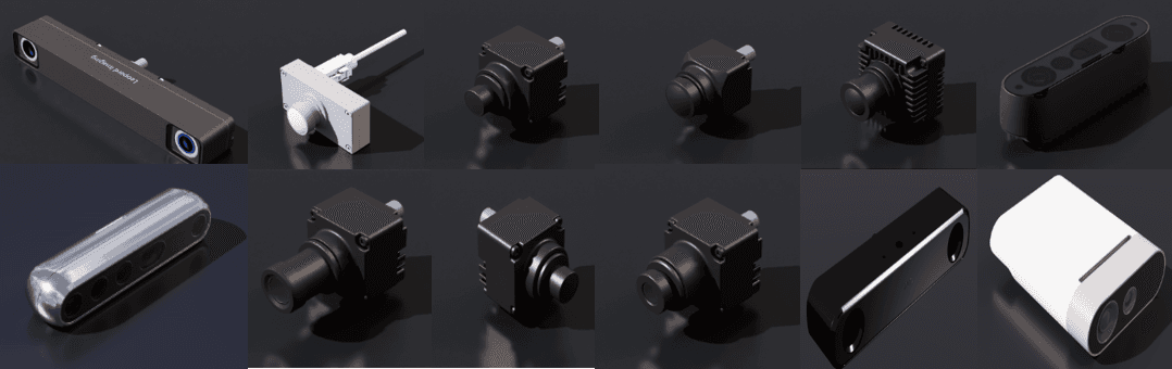
1. Overall Overview of Sensors https://docs.isaacsim.omniverse.nvidia.com/latest/sensors/index.html Isaac Sim’s sensor system is divided into six categories and supports simulation of various sensors that are physics-based, RTX-based, camera-based, and applicable to real robots. Each category is used for the following purposes. 2. Camera Sensors https://docs.isaacsim.omniverse.nvidia.com/latest/sensors/isaacsim_sensors_camera.html The basic RGB/Depth cameras used in Isaac Sim can be simulated similar to real lenses and support various annotator outputs. What are Annotators? In Isaac Sim, an annotator automatically generates additional ground-truth data streams beyond the images produced by a sensor. This data is extremely useful for machine learning training, robot perception, and validation. Major Annotator Types and Descriptions: In Isaac Sim, this data can be output as .png, .json, .npy, ROS messages, etc., and can be controlled via Python API or Action Graph. Supported Features: Configure focal length, FOV, resolution, sensor size Apply lens distortion models (pinhole, fisheye, etc.) Integration with render products for rendering Annotator support: RGB, Depth, Normals, Motion Vectors, Instance Segmentation, etc. Creation and control via Python or GUI Example Uses: Simulation for object recognition data collection Synthetic data generation for deep-learning-based vision training RGB-D data output for ROS/SLAM integration 3. RTX Sensors https://docs.isaacsim.omniverse.nvidia.com/latest/sensors/isaacsim_sensors_rtx.html A family of high-precision sensors for distance/velocity detection using NVIDIA RTX acceleration. It consists of lidar, radar, and visual annotators. Subcomponents: RTX Lidar Sensor: Outputs point clouds; adjustable rotation angle, FOV, and ray density RTX Radar Sensor: Extracts distance + velocity (simulates Doppler effect) RTX Sensor Annotators: Output properties for visualization Visual/Non-Visual Materials: Materials for sensor response Example Uses: Autonomous vehicles, AMRs, and robot ranging Comparing detection capabilities across sensor types Visual Materials (Sensor Materials for Visual Response) Simulate the visual properties of object surfaces that RTX sensors detect (e.g., reflectance, absorption). These affect both rendering and sensor response; a total of 21 fixed material types are provided. Non-Visual Sensor Material Properties Do not affect rendering, but control detectability and reflectance strength for RTX sensors. This allows specific objects to be detected or ignored in simulation. Purposes: Improve accuracy of sensor tests Make certain objects detectable or hidden Keep visual material intact while altering only sensor response 4. Physics-Based Sensors https://docs.isaacsim.omniverse.nvidia.com/latest/sensors/isaacsim_sensors_physics.html Sensors implemented based on interactions in the physics engine (PhysX) to sense internal robot states or external contacts. Supported Sensors: Articulation Joint Sensor: Full joint state sensing (position/velocity/effort) Contact Sensor: Ground contact, collision detection Effort Sensor: Measures joint torque only IMU Sensor: Inertial data (acceleration, gyro) Proximity Sensor: Simple detection of whether an object exists within a certain range (True/False) Example Uses: Evaluating robot walking stability Force/torque analysis for manipulators Landing detection, fall detection 5. PhysX SDK Sensors https://docs.isaacsim.omniverse.nvidia.com/latest/sensors/isaacsim_sensors_physx.html Lightweight distance sensors using the PhysX SDK’s raycast functionality. Supported Items: Generic Sensor: Custom ray-based sensing PhysX Lidar: Fixed lidar simulation (low-cost version) Lightbeam Sensor: One-way detector similar to a laser Example Uses: Simple distance-based obstacle detection Environment change detection Low-compute-cost sensor simulation 6. Camera and Depth Sensors (USD Assets) https://docs.isaacsim.omniverse.nvidia.com/latest/assets/usd_assets_camera_depth_sensors.html A collection of USD-based camera and depth sensor assets modeled after frequently used real sensors. Included Sensors: Example Uses: Sim-to-Real consistency testing with specific real sensors Replicating real sensor positions/fields of view 7. Non-Visual Sensors (USD Assets) https://docs.isaacsim.omniverse.nvidia.com/latest/assets/usd_assets_nonvisual_sensors.html A collection of assets for digital twins of non-visual sensors (IMU, force, contact, etc.). Asset Contents: Example Uses: Extracting internal robot physical quantities (forces, acceleration) Motion estimation, control feedback system development
Nov 4, 2025
